User Guide
Installation
pip install -e /path/to/mpmath_fft
Or run directly from the repo root (the package is importable as-is):
cd mpmath_fft/
python -c "from mpmath_fft import fft; print(fft(...))"
Dependencies: mpmath >= 1.3,
numpy >= 1.24, Python >= 3.10.
Quick start
import mpmath as mp
import numpy as np
from mpmath_fft import fft, ifft, build_plan

# 1D transform
x = np.array([mp.mpc(i, 0) for i in range(16)], dtype=object)
y = fft(x)
z = ifft(y)          # round-trip: z ~ x

# ND axis-aware
x2d = np.empty((3, 4), dtype=object)
# ... fill with mpc values ...
y2d = fft(x2d, axis=-1)

# Explicit plan (cached by N and mp.mp.dps)
plan = build_plan(128)
Real-valued transforms
rfft(x, n=None, axis=-1) computes the forward DFT of real-valued input
(mp.mpf) and returns only the non-redundant half of the spectrum:
indices 0..n//2, shape (..., n//2 + 1, ...). If n > len(x) the
input is zero-padded; if n < len(x) it is truncated.
irfft(x, n=None, axis=-1) reconstructs the full Hermitian-symmetric
spectrum from the half-spectrum, computes the inverse DFT, and returns
the real part (mp.mpf). Default output length is 2*(M-1) where
M = x.shape[axis].
hfft / ihfft are re-expressed in terms of rfft / irfft via the
identities (verified against numpy.fft):
ihfft(x, n) = conj(rfft(x, n)) / n_used
hfft(X, n)  = n_used * irfft(conj(X), n=n)
where n_used is the explicit n parameter or len(x) / 2*(M-1).
rfftfreq(n, d=1.0) returns the non-negative frequencies
f_k = k/(n*d) for k = 0..n//2.
These follow numpy.fft conventions exactly, including the n padding/
truncation semantics and Hermitian half-spectrum layout.
Algorithm coverage
The planner selects the fastest available decomposition for each transform size:
N |
Strategy |
Cost |
|---|---|---|
1 |
Identity (no-op) |
O(1) |
3, 4 |
Unrolled hard-coded DFT |
O(1) |
5-31 |
O(N^2) naive DFT (non-pow2) |
O(N^2) |
2^n |
Iterative radix-2 DIT |
O(N log N) |
>=32 |
Bluestein chirp-Z -> power-of-2 convolution (prime) |
O(N log N) |
>=32 |
Cooley-Tukey with recursive decomposition (composite) |
O(N log N) |
Bluestein chirp-Z
For prime N, the DFT is recast as a convolution padded to the next
power of 2 (M = 2^p >= 2N+1). The convolution is computed via
three radix-2 FFTs of size M. This handles any N, not just
highly-composite sizes.
Plan structure
build_plan(N) returns an 8-tuple of flat numpy arrays following
the pynalgo.fft convention:
Node type codes: 0=ident, 1=N=3, 2=N=4, 3=naive, 4=radix2, 5=CT, 6=Bluestein.
Node ids are pre-order (root=0). The stack executor uses dynamically-resized numpy arrays.
Precision behavior
Plans are cached by (N, mp.mp.dps) because twiddle factors are
computed at the current mpmath precision. Changing mp.mp.dps
after building a plan does not retroactively change the plan’s
precision - a new plan is built on the next call.
The cache holds at most 128 entries. When full, the oldest entry
is evicted (FIFO). Use clear_plan_cache() to discard all
cached plans; useful after a bulk computation or precision change.
Thread safety
build_plan() uses double-checked locking: concurrent calls for
different (N, dps) keys can build plans in parallel, and cache
inserts are serialised. clear_plan_cache() acquires the same lock.
fft(), ifft(), rfft(), irfft() are also safe to call from
multiple threads. Each copies its input into a private buffer,
reads the cached plan (read-only after construction), and executes
on that buffer without shared mutable state.
Error at dps=D scales approximately as 10^(-D) * sqrt(N log N). Observed round-trip errors:
dps |
N=100 threshold |
|---|---|
15 |
1e-11 |
50 |
2e-47 |
100 |
5e-95 |
Comparison targets
dps=15: Compare against
numpy.fft(float64 reference, ~1e-15 floor).dps >= 50: Compare against naive O(N^2) DFT computed at the same precision. Never compare high-precision output against numpy - float64 masks the true error.
Key differences from pynalgo.fft
Aspect |
pynalgo.fft |
mpmath_fft |
|---|---|---|
Precision |
float64 / complex128 |
arbitrary (mpmath mpc) |
Array dtype |
complex128 |
object |
Compilation |
@JIT / @JITG |
pure Python |
Twiddle exp() |
|
|
Plan cache |
JIT cache handles reuse |
explicit |
Usage examples
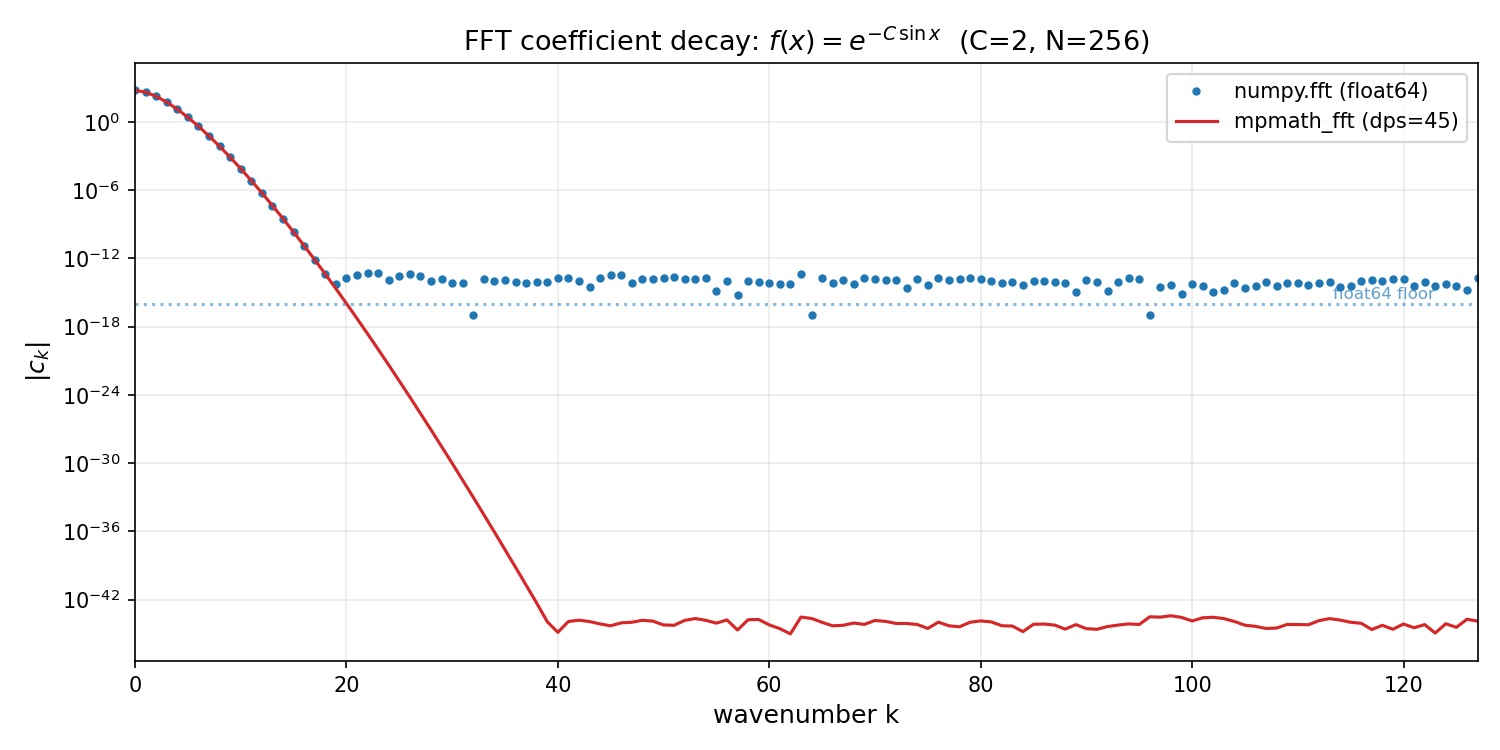
``usage/demo.py`` - precision convergence table, 2D transform, prime-size Bluestein, high-precision round-trip with 50-digit output.
``usage/spectral_decay.py`` - plots
|FFT(f)| for f(x) = exp(-C sin x) on semilog axes, comparing
numpy.fft (float64 noise floor at ~1e-15) against mpmath_fft at
dps=45.
Testing
bash run_tests.sh
Runs pytest, mypy (on mpmath_fft/, tests/, benchmarks/), and ruff
(on mpmath_fft/, tests/, usage/, benchmarks/).
Tests cover:
Correctness vs
numpy.fftat dps=15 (pow2, composite, prime)Round-trip identity at dps=15, 50, 100
Naive DFT comparison at dps=50, 100
Precision convergence: 6 dps levels (15->100), error must decrease monotonically
Linearity:
fft(a*x + b*y) = a*fft(x) + b*fft(y)2D/3D/4D axis dispatch and round-trip
Plan cache reuse and precision invalidation
Input validation
All public functions validate their inputs and raise clear errors:
Non-ndarray input ->
TypeError("requires numpy ndarray, got ...")Wrong dtype ->
TypeError("requires dtype=object array, got ...")Wrong element type ->
TypeError("requires array elements of type mp.mpc, got ...")Non-integer axis ->
TypeError("axis must be int, got ...")Out-of-bounds axis ->
ValueError("axis N out of bounds for array with D dimensions")Empty transform axis ->
ValueError("requires at least 1 element along transform axis")build_plan(0)->ValueError("requires positive N, got 0")fftfreq(0)/rfftfreq(0)->ValueError
Number theory helpers
Self-contained in the kernels module (_kernels.py, no pynalgo dependency):
_get_prime_factors(N)- prime factorization_is_prime(N)- primality test (6k+(-)1 wheel)_is_pow2(N)- power-of-2 check_balanced_split(N)- find N = N1*N2 with N1 ~ sqrt(N), N1’s prime factors a subset of N’s
Limitations
No JIT compilation. The use case is correctness at arbitrary precision, not speed.
Precision scales wall time. mpmath arithmetic cost grows with
dps. A Bluestein FFT of prime N ~ 100 at dps=100 is ~10x slower than at dps=15.Object arrays only. numpy vectorized operations (
np.dot,np.exp) do not dispatch to mpmath on object arrays. All arithmetic is done element-by-element in Python loops.No GPU or parallel execution. Pure Python with no CUDA, OpenCL, or multiprocessing. Threads can call transforms concurrently on different inputs, but a single transform uses one core.
No in-place transforms. All public functions copy input before operating. The internal executor operates in-place on a private buffer.
mp.mpc format strings.
mp.mpc.__format__does not accept format specs (e.g..1e). Usefloat(val)ormp.nstr()for printing.
References
Cooley, J. W. & Tukey, J. W. (1965). An algorithm for the machine calculation of complex Fourier series. Math. Comp., 19(90), 297-301.
Bluestein, L. I. (1970). A linear filtering approach to the computation of discrete Fourier transform. IEEE Trans. Audio Electroacoustics, 18(4), 451-455.
Chu, E. & George, A. (1999). Inside the FFT Black Box. CRC Press.
Johnson, S. G. & Frigo, M. (2009). Implementing FFTs in practice. In Fast Fourier Transforms (C. S. Burrus, ed.), Connexions.
Frigo, M. & Johnson, S. G. (2005). The design and implementation of FFTW3. Proc. IEEE, 93(2), 216-231.